Titanic Kaggle Machine Learning Competition With R - Part 3: Selecting and Tuning The Model

Tutorial Table of Contents

Part 1: Knowing and Preparing the Data
Part 2: Learning From Data
Part 3: Selecting and Tuning the Model

In part 2, we tried different models to predict passenger survival on Titanic. We know that an increase in training accurracy, does not always result in increase in the Kaggle score. Herein, we discuss more details.

Overfitting & Cross-validation

In the machine learning practice, we are intersted in predictive models capable of predicting something in the real world. We’d like to predict something given all we know about the instance. So, our models should be capable of being generalized to cover real-world scenarios.

When we check the accuracy of our predictions against the training data and maximize our accuracy in this setting, there is a risk of overfitting the training data, meaning we have captured so much of the outliers, exceptions, and particularities of the training data that the resulting model cannot be generalized anymore. This is what has happened with our sex.class.age.tree model.

What can be done to avoid overfitting? We can create different versions of the training data, keeping part of the training data as test set, evaluate our model, and pick the model that performs best, on average. This is called cross-validation. Let’s see a practical example of cross-validation.

K-fold Cross Validation

One of the popular methods of cross validation is K-fold cross validation. In this method, the training data is split into k partitions. Each time, we leave out one of the partitions and train the model on the rest, then test and measure the performance on the partition not used for training. To determine the model performance, average performance of all the k runs will be used.

1
2
3
4
5
set.seed(100)
cvCtrl <- trainControl(method= "cv", number = 10) # use 10-fold cross validation
sex.class.age.tree <- train(Survived ~ Sex.factor + Pclass.factor + Age, 
                            data= train.data.impute, method= "rpart",
                            trControl= cvCtrl)

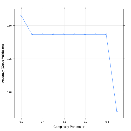
trainControl function is used to create a 10-fold cross validation control object. This object is then passed to the train function. Decision trees are controlled by cp (complexity parameter), which tells the algorithm to stop when the measure (accuracy here) does not improve by this factor. So, we are using 10-fold cross validation to find an appropriate cp.

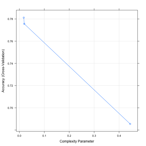
plot.train and print.train show the details of training, i.e. how accuracy changed by changing cp.

1
plot.train(sex.class.age.tree)

plot of chunk unnamed-chunk-3

1
print.train(sex.class.age.tree)

## CART 
## 
## 891 samples
##  14 predictor
##   2 classes: '0', '1' 
## 
## No pre-processing
## Resampling: Cross-Validated (10 fold) 
## Summary of sample sizes: 801, 802, 802, 802, 801, 802, ... 
## Resampling results across tuning parameters:
## 
##   cp          Accuracy   Kappa      Accuracy SD  Kappa SD  
##   0.01754386  0.7812189  0.5274347  0.02995344   0.06533745
##   0.01949318  0.7755882  0.5136375  0.02902230   0.06529576
##   0.44444444  0.6854835  0.2363187  0.07256908   0.25009530
## 
## Accuracy was used to select the optimal model using  the
##  largest value.
## The final value used for the model was cp = 0.01754386.

1
plot.decision.tree(sex.class.age.tree$finalModel)

plot of chunk unnamed-chunk-3

1
conMat$table

##           Reference
## Prediction   0   1
##          0 511 125
##          1  38 217

1
percent(conMat$overall["Accuracy"])

## Accuracy 
##    81.71

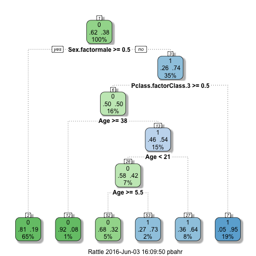
The default value for cp is 0.01 and that’s why our tree didn’t change compared to what we had at the end of part 2.

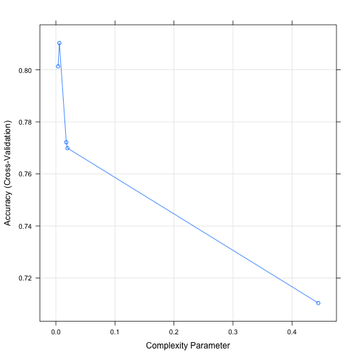
Another parameter to control the training behavior is tuneLength, which tells how many instances to use for training. The default value for tuneLength is 3, meaning 3 different values will be used per control parameter. Since we only have one control parameter (cp), it will try three different trees with different values for cp. Let’s change this default to see what happens.

1
2
3
4
5
cvCtrl <- trainControl(method= "cv", number = 10)
sex.class.age.tree.cv <- train(Survived ~ Sex.factor + Pclass.factor + Age, 
                            data= train.data.impute, method= "rpart",
                            trControl= cvCtrl,
                            tuneLength= 5)

1
plot.train(sex.class.age.tree.cv)

plot of chunk unnamed-chunk-5

1
print.train(sex.class.age.tree.cv)

## CART 
## 
## 891 samples
##  14 predictor
##   2 classes: '0', '1' 
## 
## No pre-processing
## Resampling: Cross-Validated (10 fold) 
## Summary of sample sizes: 802, 801, 802, 802, 803, 801, ... 
## Resampling results across tuning parameters:
## 
##   cp           Accuracy   Kappa      Accuracy SD  Kappa SD  
##   0.003654971  0.8013174  0.5712676  0.02974081   0.06310653
##   0.005847953  0.8103067  0.5846073  0.02935917   0.06355443
##   0.017543860  0.7721797  0.5076753  0.02739884   0.07483216
##   0.019493177  0.7699197  0.5007175  0.02710966   0.07336329
##   0.444444444  0.7103816  0.3041572  0.07976966   0.26233191
## 
## Accuracy was used to select the optimal model using  the
##  largest value.
## The final value used for the model was cp = 0.005847953.

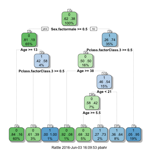
As we see in the output, 5 different trees with different cps have been tried and the cp with highest accuracy has been picked. Because the resulting cp is lower that the default value, we get a different tree this time.

1
plot.decision.tree(sex.class.age.tree.cv$finalModel)

plot of chunk unnamed-chunk-6

1
2
sex.class.age.survival.cv <- predict(sex.class.age.tree.cv, train.data.impute)
conMat <- confusionMatrix(sex.class.age.survival.cv, train.data.impute$Survived)

1
conMat$table

##           Reference
## Prediction   0   1
##          0 511 113
##          1  38 229

1
percent(conMat$overall["Accuracy"])

## Accuracy 
##    83.05

1
2
3
4
5
6
sex.class.age.solution.cv <- get.solution(sex.class.age.tree.cv, test.data.impute)

if(!file.exists("output/new versions/sex_class_age_tl_cv.csv"))
    write.csv(sex.class.age.solution.cv, 
              file= "output/new versions/sex_class_age_tl_cv.csv", 
              row.names= FALSE)

So, we went from 81.71% in training accuracy to 83.05%. Now, we have both higher training accuracy and better Kaggle score (0.75598). What if we continue increasing tuneLength?

1
2
3
4
5
cvCtrl <- trainControl(method= "cv", number = 10)
sex.class.age.tree.cv.tl <- train(Survived ~ Sex.factor + Pclass.factor + Age, 
                            data= train.data.impute, method= "rpart",
                            trControl= cvCtrl,
                            tuneLength= 10)

1
plot.train(sex.class.age.tree.cv.tl)

plot of chunk unnamed-chunk-8

1
print.train(sex.class.age.tree.cv.tl)

## CART 
## 
## 891 samples
##  14 predictor
##   2 classes: '0', '1' 
## 
## No pre-processing
## Resampling: Cross-Validated (10 fold) 
## Summary of sample sizes: 802, 802, 802, 802, 802, 802, ... 
## Resampling results across tuning parameters:
## 
##   cp          Accuracy   Kappa      Accuracy SD  Kappa SD  
##   0.00000000  0.8147815  0.5996698  0.03377014   0.07021752
##   0.04938272  0.7868165  0.5417724  0.03337273   0.07249247
##   0.09876543  0.7868165  0.5417724  0.03337273   0.07249247
##   0.14814815  0.7868165  0.5417724  0.03337273   0.07249247
##   0.19753086  0.7868165  0.5417724  0.03337273   0.07249247
##   0.24691358  0.7868165  0.5417724  0.03337273   0.07249247
##   0.29629630  0.7868165  0.5417724  0.03337273   0.07249247
##   0.34567901  0.7868165  0.5417724  0.03337273   0.07249247
##   0.39506173  0.7868165  0.5417724  0.03337273   0.07249247
##   0.44444444  0.6710861  0.1859201  0.07272003   0.24110245
## 
## Accuracy was used to select the optimal model using  the
##  largest value.
## The final value used for the model was cp = 0.

1
plot.decision.tree(sex.class.age.tree.cv.tl$finalModel)

plot of chunk unnamed-chunk-8

1
2
sex.class.age.survival.cv.tl <- predict(sex.class.age.tree.cv.tl, train.data.impute)
conMat <- confusionMatrix(sex.class.age.survival.cv.tl, train.data.impute$Survived)

1
conMat$table

##           Reference
## Prediction   0   1
##          0 486  64
##          1  63 278

1
percent(conMat$overall["Accuracy"])

## Accuracy 
##    85.75

1
2
3
4
5
6
sex.class.age.solution.cv.tl <- get.solution(sex.class.age.tree.cv.tl, test.data.impute)

if(!file.exists("output/new versions/sex_class_age_tl_cv_10.csv"))
    write.csv(sex.class.age.solution.cv, 
              file= "output/new versions/sex_class_age_tl_cv_10.csv" , 
              row.names= FALSE)

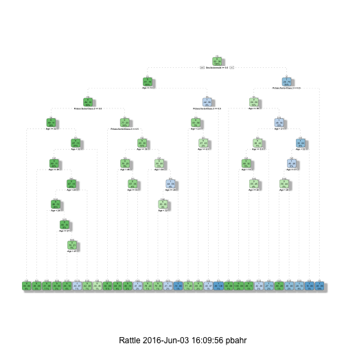
When submitted to Kaggle, our increased training accuracy (85.75%) did not translate to increased Kaggle score, as we could expect. This is another example of overfitting, where our model couldn’t be generalized to accurately predict survival for unknown test data.

So, in general it is not advisable to maximize tuneLength, because high values may result in overfitting, as we may get too many similar trees that won’t help. The result in this case is a complete tree with branches not pruned and some nodes too sepcific.

Putting it together

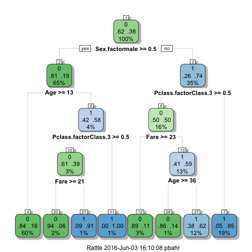
Let’s bring Fare back with all the tuning in place.

1
2
3
4
5
6
7
8
cvCtrl <- trainControl(method= "cv", number = 10)
sex.class.fare.age.tree <- train(Survived ~ Sex.factor + Pclass.factor + Fare + Age, 
                                 data= train.data.impute, method= "rpart",
                                 trControl= cvCtrl,
                                 tuneLength= 5)

sex.class.fare.age.survival <- predict(sex.class.fare.age.tree, train.data.impute)
conMat <- confusionMatrix(sex.class.fare.age.survival, train.data.impute$Survived)

1
conMat$table

##           Reference
## Prediction   0   1
##          0 497  91
##          1  52 251

1
percent(conMat$overall["Accuracy"])

## Accuracy 
##    83.95

1
plot.decision.tree(sex.class.fare.age.tree$finalModel)

plot of chunk unnamed-chunk-10

1
2
3
4
sex.class.fare.age.solution <- get.solution(sex.class.fare.age.tree, test.data.impute)

write.csv(sex.class.fare.age.solution, 
          file= "output/new versions/sex_class_fare_age_cv_tl.csv" , row.names= F)

1
plot.train(sex.class.fare.age.tree)

plot of chunk unnamed-chunk-11

1
print.train(sex.class.fare.age.tree)

## CART 
## 
## 891 samples
##  14 predictor
##   2 classes: '0', '1' 
## 
## No pre-processing
## Resampling: Cross-Validated (10 fold) 
## Summary of sample sizes: 802, 802, 802, 802, 802, 802, ... 
## Resampling results across tuning parameters:
## 
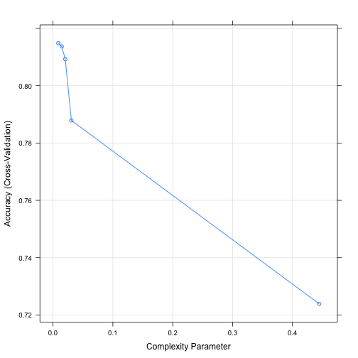
##   cp          Accuracy   Kappa      Accuracy SD  Kappa SD  
##   0.00877193  0.8148689  0.5954804  0.04310355   0.10092410
##   0.01461988  0.8137203  0.5962228  0.04669299   0.10468162
##   0.02046784  0.8092509  0.5874807  0.04173675   0.09049861
##   0.03070175  0.7878901  0.5425921  0.03053194   0.06971850
##   0.44444444  0.7238577  0.3533356  0.07676797   0.24606106
## 
## Accuracy was used to select the optimal model using  the
##  largest value.
## The final value used for the model was cp = 0.00877193.

This time we get better training accuracy than that of the model without Fare (83.95% compared to 83.05%). Our Kaggle score has improved to 0.7799 from 0.75598.

It should be noted that the best score we have had up to this point is for the model using Sex, Pclass, and Fare. I guess that it is because of the inherent errors in imputing the missing values for Age. I will discuss different strategies for imputing the missing values and compare their results. So, see you next time.