Titanic Kaggle Machine Learning Competition With R - Part 2: Learning From Data

Tutorial Table of Contents

Part 1: Knowing and Preparing the Data
Part 2: Learning From Data
Part 3: Selecting and Tuning the Model

Machine Learning

In part 1 of this tutorial, we analyzed the data and prepared it for machine learning. Now, we are ready for some action.

Quick Intro

We are interested in predicting an outcome (response) variable, given the other features (predictors) of our data points. This is called supervised learning, there is a set of oucomes in the training data to learn from and there will be a result for each given data point at the end. This is in contrast to unsupervised learning, where there is no response variable and the observations are grouped together based on a measure of similarity.

The response variable is categorical in this case. There are two classes of passengers, people who survived and people who did not. This type of problems is called classification, compared to regression problems where we predict a quantitative response.

Decision Trees

Back to the data, we see that only 38.38% of people survived. So, if we start off by classifying everybody as Survived= 0, we will be wrong by 38%. Moreover, if we partition by gender and label females as Survived= 1 and males as Survived= 0, we will be wrong by 25.8 for women and 18.89 for men. Overall, our error will be 21.32%, which is way better that the previous 38%.

This is exactly the way decision trees work. In each round, the algorithm picks the best variable that improves the result in the best way, partitions data based on that vairable, and at the end labels data by the majority in each leaf. We’ll see the example below.

1
2
library(caret)
library(rpart)

caret is the umbrella package for machine learning using R. Different groups have developed different machine learning algorithms, where the signature of the methods are different. It means that it makes it hard to switch from one algorithm to the other. caret package solves this problem by unifying the interface for the main functions. rpart is one of the packages implementing the decision trees in R.

1
2
3
sex.model.tree <- train(Survived ~ Sex.factor + Pclass.factor, data= train.data, method= "rpart")
sex.class.survival <- predict(sex.model.tree, train.data)
conMat <- confusionMatrix(sex.class.survival, train.data$Survived)

1
conMat$table

##           Reference
## Prediction   0   1
##          0 468 109
##          1  81 233

1
percent(conMat$overall["Accuracy"])

## Accuracy 
##    78.68

1
plot.decision.tree(sex.model.tree$finalModel)

plot of chunk unnamed-chunk-3

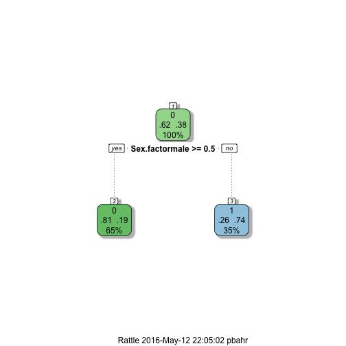
We have trained the model to predict Survived using Sex.factor and Pclass.factor using train.data and instructed caret to use decision trees implemented by rpart. Then, predicted Survived using the same training data. Here, the Survived label in the data is ignored and we are given an array of labels as the result.

Using the confusionMatrix function, we can compare our predictions to actual classes of the data. This is only possible when we know the labels in advance, i.e. training data. The important measure for us is Accuracy, which is 78.68% here. This is the percentage of the cases we got right. Note this is 1 - 21.32% we calculated before.

Although we have taken the passenger class into account, the result is not any better than just considering the gender. We have suggested Sex.factor and Pclass.factor as the predictors for Survival, but Pclass.factor didn’t get picked up by rpart as it didn’t add any new information to the decision tree.

Next, we’ve plotted the decision tree using the plot.decision.tree function from library.R to see the current situation. Different colors here represent the predicted class, which is the class of majority in that specific node. At the root, we have the complete data set and different branches represent partitioned data based on the given conditions along the way. In this example, numbers at the right of the node represent proportion of the data with Survived= 0 and the numbers at left are proportion who didn’t survive.

Now, let’s add Fare to the mix of predictors and see if we can get anything out of it.

1
2
3
sex.class.fare.tree <- train(Survived ~ Sex.factor + Pclass.factor + Fare, data= train.data, method= "rpart")
sex.class.fare.survival <- predict(sex.class.fare.tree, train.data)
conMat <- confusionMatrix(sex.class.fare.survival, train.data$Survived)

1
conMat$table

##           Reference
## Prediction   0   1
##          0 492 112
##          1  57 230

1
percent(conMat$overall["Accuracy"])

## Accuracy 
##    81.03

1
plot.decision.tree(sex.class.fare.tree$finalModel)

plot of chunk unnamed-chunk-4

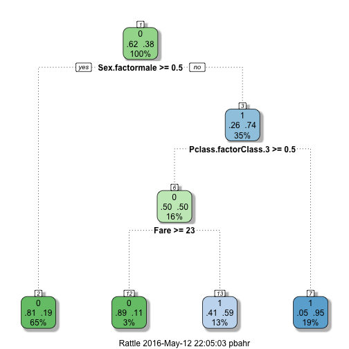
At the first glance, we have a higher accuracy rate. This may be a good sign. The decision tree have found a mix of Pclass.factor= 3 and Fare >= 23 conditions to provide a more accurate prediction. We used to predict that women survive with a 74% chance. Now, we can be more accurate. Women have a 95% chance of survival if they are not in class 3. For the women in class 3, the survival rate is 11% if the fare was more than $23, and 59% otherwise. Let’s see if it makes sense.

1
2
3
4
5
ggplot(train.data[train.data$Pclass.factor== "Class.3" & 
                      train.data$Sex.factor == "female",], 
       aes(x= Survived, y= Fare)) +
    geom_boxplot() +
    ggtitle("Class 3 women who survived paid less fare on average")

plot of chunk ml-4

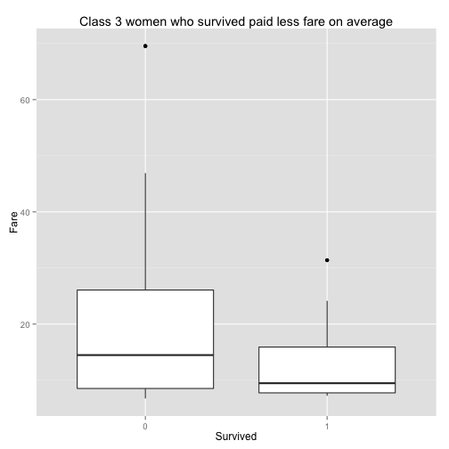
So, the decision tree discovered a special condition that makes a difference in survival. It would not be easy for us to discover on our own.

Prediction

We are almost ready for our first prediction, but we’ve got a little problem.

1
sapply(test.data[,c("Pclass.factor", "Sex.factor", "Fare")], summary)

## $Pclass.factor
## Class.1 Class.2 Class.3 
##     107      93     218 
## 
## $Sex.factor
## female   male 
##    152    266 
## 
## $Fare
##    Min. 1st Qu.  Median    Mean 3rd Qu.    Max.    NA's 
##   0.000   7.896  14.450  35.630  31.500 512.300       1

Checking the Fare predictor, we see that it has a missing value in the test data. Since our decision tree needs to know this value, it cannot predict Survive for this data point. So, let’s impute the missing value with the median for the Fare.

1
2
3
4
full.data$Fare[is.na(full.data$Fare)] <- median(full.data$Fare, na.rm = T)
test.data <- full.data[(train.len+1):nrow(full.data), ]

sex.class.fare.solution <- get.solution(sex.class.fare.tree, test.data)

Then, we have predicted the Survive class using get.solution function from library.R. It uses predict function and the given decision tree to predict the outcome for the given test data and builds the data frame the way Kaggle expects. Check the code below.

## function (tree, data) 
## {
##     my_prediction <- predict(tree, data)
##     my_solution <- data.frame(PassengerId = data$PassengerId, 
##         Survived = my_prediction)
##     my_solution
## }

And finally, we write the prediction to a CSV file to be submitted to Kaggle.

1
2
3
# Write your solution to a csv file with the name my_solution.csv
if (!file.exists("output/new versions/sex_class_fare.csv"))
    write.csv(sex.class.fare.solution, file= "output/new versions/sex_class_fare.csv" , row.names= FALSE)

When I submitted this file to Kaggle, I got a score of .78469. It is right above the benchmark titled “Gender, Price, and Class Based Model” (0.7799).

Dealing With Missing Data

We already know that age can be a good predictor for survival. We also know that the decision tree algorithm cannot predict the outcome using the predictors with missing values. From our numerical analysis, we know there are 177 instances with Age missing. So, we need to impute the missing values.

Although we can still use the median age as the imputed value, it would not an optimal strategy. It is highly unlikely that everybody with a missing value for age is actually of the same age. We need to use a better estimate if possible.

We can use the average age of similar people as the missing value for age. The K-Nearest Neighbors (KNN) algorithm does this for us. We will use the value for Pclass, Age, SibSp, Parch, Fare to find similar nodes (neighbors) and use their mean age as the imputed age. We use the default value of 5 for k.

1
2
3
4
# Pick columns to define neighbors
relevant.vars <- c(2, 5:7, 9)
# Data set to impute from
impute.data <- full.data[,relevant.vars]

1
names(full.data)[relevant.vars]

## [1] "Pclass" "Age"    "SibSp"  "Parch"  "Fare"

1
2
3
4
5
6
7
8
9
10
11
12
13
14
# Prepare the preProcess object
pp <- preProcess(impute.data, method = c("knnImpute"))

# get imputed age, and the original mean and standard deviation
imputedAge <- predict(pp, newdata = impute.data)$Age
meanAge <- pp$mean["Age"] 
stdAge <- pp$std["Age"]

# back to original scale
imputedAge <- imputedAge * stdAge + meanAge

full.data.impute <- full.data
selector <- is.na(full.data$Age)
full.data.impute$Age[selector] <- imputedAge[selector]

preProcess method of caret package is used to impute the missing values with method= "knnImpute". Because preProcess centers and scales the data in the process of knnImpute, we need to convert them back to the original scale to be used as valid age values. The Age variable is updated to the imputed values for the people with missing Age.

1
2
3
4
train.data.impute <- full.data.impute[1:train.len, ]
test.data.impute <- full.data.impute[(train.len+1):nrow(full.data.impute), ]
# Add the outcome column
train.data.impute$Survived <- train.outcome

1
2
3
4
ggplot(train.data.impute, aes(x= Pclass.factor, y= Age, color= Survived)) +
    geom_violin() +
    geom_jitter(alpha= .5) +
    ggtitle("Age Still Matters!")

plot of chunk unnamed-chunk-7

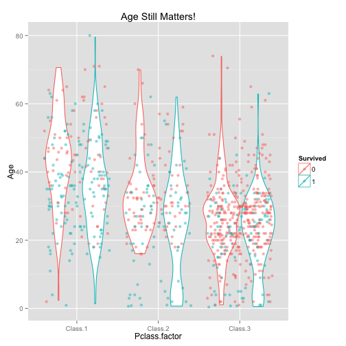
The differences still exist in the survival rate for people in different age ranges. Let’s check the decision tree of Sex, Pclass, and Age instead of Fare.

1
2
3
sex.class.age.tree <- train(Survived ~ Sex + Pclass + Age, data= train.data.impute, method= "rpart")
sex.class.age.survival <- predict(sex.class.age.tree, train.data.impute)
conMat <- confusionMatrix(sex.class.age.survival, train.data.impute$Survived)

1
conMat$table

##           Reference
## Prediction   0   1
##          0 511 125
##          1  38 217

1
percent(conMat$overall["Accuracy"])

## Accuracy 
##    81.71

1
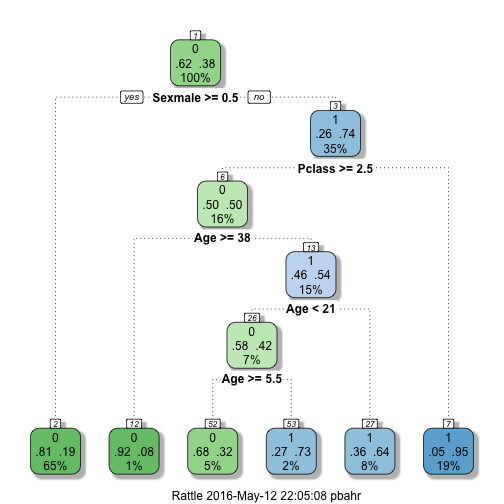
plot.decision.tree(sex.class.age.tree$finalModel)

plot of chunk unnamed-chunk-8

1
2
3
4
sex.class.age.solution <- get.solution(sex.class.age.tree, test.data.impute)

if (!file.exists("output/new versions/sex_class_age.csv"))
    write.csv(sex.class.age.solution, file= "output/new versions/sex_class_age.csv" , row.names= FALSE)

We have a more detailed tree this time. Age especially matters among class 3 females, who survied by 50%. In this group, people over 38 survived by 8%, 21-38 year by 64%, 5.5-21 years by 32% and less than 5.5 by 73%.

We have an increase in accuracy for training data compared to using Sex, Pclass, and Fare from 81.03 to 81.71, but when submitted to Kaggle the score was .74641 as opposed to .78469 we had before. What is going on here?

We will look into this issue in part 3.